Tutorial (observational data set)

This package is designed to aid in the efficient analysis of large datasets, such as GAIA DR3.

Tutorial dataset

In the following, we will subset from the GAIA data release 3. The reduced dataset contains 100000 randomly selected entries only. The reduced dataset can be downloaded here. Check Supported Datasets for an incomplete list of supported datasets and requirements for support of new datasets. A tutorial for a cosmological simulation can be found here.

It uses the dask library to perform computations, which has several key advantages:

very large datasets which cannot normally fit into memory can be analyzed,
calculations can be automatically distributed onto parallel 'workers', across one or more nodes, to speed them up,
we can create abstract graphs ("recipes", such as for derived quantities) and only evaluate on actual demand.

Loading an individual dataset

Here we use the GAIA data release 3 as an example. In particular, we support the single HDF5 version of DR3.

The dataset is obtained in HDF5 format as used at ITA Heidelberg. We intentionally select a small subset of the data to work with. Choosing a subset means that the data size is small and easy to work with. We demonstrate how to work with larger data sets at a later stage.

First, we load the dataset using the convenience function load() that will determine the appropriate dataset class for us:

Missing units

Below snippet will report missing units for some fields. This is expected. Those fields that cannot have their units determined automatically at this point and carry the unit unknown. See Units for more information.

Loading a dataset

>>> from scida import load
>>> ds = load("gaia_dr3_subset100000.hdf5", units=True) #(1)!
>>> ds.info() #(2)!
class: DatasetWithUnitMixin
source: /home/cbyrohl/data/testdata-scida/gaia_dr3_subset100000.hdf5
=== Unit-aware Dataset ===
==========================
=== data ===
+ root (fields: 27, entries: 100000)
============

The units=True argument will attach code units to all fields (default). Alternative choices are False to go without units and cgs for cgs units. The current default is False, which will change to True in the near future.
Call to receive some information about the loaded dataset.

The dataset is now loaded, and we can inspect its contents, specifically its container and fields loaded. We can access the data in the dataset by using the data attribute, which is a dictionary of containers and fields.

We have a total of 27 fields available, which are:

Available fields

>>> ds.data.keys()
['pmdec',
 'distance_gspphot',
...
 'distance_gspphot_upper',
 'pmra_error']

Let's take a look at some field in this container:

Inspecting a field

>>> ds.data["dec"]
dask.array<mul, shape=(100000,), dtype=float64, chunksize=(100000,), chunktype=numpy.ndarray> <Unit('degree')>

The field is a dask array, which is a lazy array that will only be evaluated when needed. How these lazy arrays and their units work and are to be used will be explored in the next section.

Dask arrays and units

Dask arrays

Dask arrays are virtual entities that are only evaluated when needed. If you are unfamiliar with dask arrays, consider taking a look at this 3-minute introduction.

They are not numpy arrays, but they can be converted to them, and have most of their functionality. Within dask, an internal task graph is created that holds the recipes how to construct the array from the underlying data.

In general, fields can be also be stored in flat or more nested structures, depending on the dataset.

We can trigger the evaluation of the dask array by calling compute() on it:

Evaluating a dask array

>>> ds.data["dec"].compute()
array([ 0.86655069,  1.15477218,  2.14207063, ..., -1.5291509 ,
       -1.30061261, -0.88984633]) <Unit('degree')>

However, directly evaluating dask arrays is strongly discouraged for large datasets, as it will load the entire dataset into memory. Instead, we will reduce the datasize by running desired analysis/reduction within dask before calling compute(), which we present in the next section.

Units

If passing units=True (default) to load(), the dataset will be loaded with code units attached to all fields. These units are attached to each field / dask array. Units are provided via the pint package. See the pint documentation for more information. Also check out this page for more unit-related examples.

In short, each field, that is represented by a modified dask array, has a magnitude (the dask array without any units attached) and a unit. These can be accessed via the magnitude and units attributes, respectively.

Accessing the magnitude and units of a field

>>> ds.data["dec"].magnitude.compute(), ds.data["dec"].units
(dask.array<mul, shape=(100000,), dtype=float64, chunksize=(100000,), chunktype=numpy.ndarray>,
 <Unit('degree')>)

When defining derived fields from dask arrays, the correct units are automatically propagated to the new field, and dimensionality checks are performed. Importantly, the unit calculation is done immediately, thus allowing to directly see the resulting units and any dimensionality mismatches.

Analyzing the data

Computing a simple statistic on (all) objects

The fields in our data object behave similar to actual numpy arrays.

As a first simple example, let's calculate the mean declination of the stars. Just as in numpy we can write

Calculating the mean declination

>>> dec = ds.data["dec"]
>>> task = dec.mean()
>>> task
dask.array<mean_agg-aggregate, shape=(), dtype=float64, chunksize=(), chunktype=numpy.ndarray> <Unit('degree')>

Note that all objects remain 'virtual': they are not calculated or loaded from disk, but are merely the required instructions, encoded into tasks.

We can request a calculation of the actual operation(s) by applying the .compute() method to the task.

>>> meandec = task.compute()
>>> meandec
-18.433358575323904 <Unit('degree')>

As an example of calculating something more complicated than just sum(), let's do the usual "poor man's projection" via a 2D histogram.

To do so, we use da.histogram2d() of dask, which is analogous to numpy.histogram2d(), except that it operates on a dask array. We discuss more advanced and interactive visualization methods here.

>>> import dask.array as da
>>> import numpy as np
>>> x = ds.data["l"]
>>> y = ds.data["b"]
>>> nbins = (360, 180)
>>> extent = [0.0, 360.0, -90.0, 90.0]
>>> xbins = np.linspace(*extent[:2], nbins[0] + 1)
>>> ybins = np.linspace(*extent[-2:], nbins[1] + 1)
>>> hist, xbins, ybins = da.histogram2d(x, y, bins=[xbins, ybins])
>>> im2d = hist.compute() #(1)!
>>> import matplotlib.pyplot as plt
>>> from matplotlib.colors import LogNorm
>>> plt.imshow(im2d.T, origin="lower", norm=LogNorm(), extent=extent, interpolation="none")
>>> plt.xlabel("l [deg]")
>>> plt.ylabel("b [deg]")
>>> plt.show()

The compute() on im2d results in a two-dimensional array which we can display.

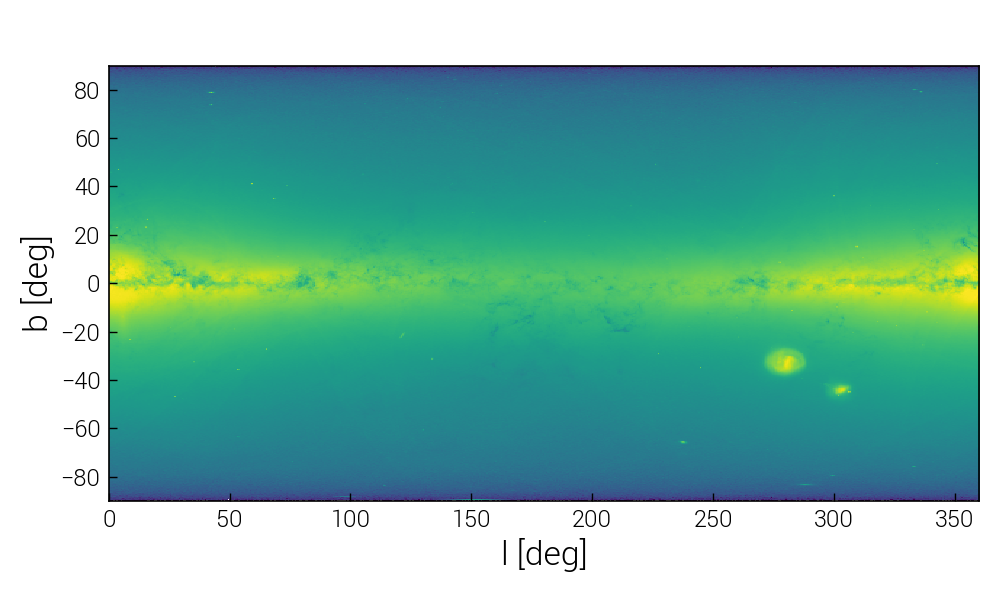
Info

Above image shows the histogram obtained for the full data set.

FITS files

Observations are often stored in FITS files. Support in scida is work-in-progress and requires the astropy package. Here we show use of the SDSS DR16.

SDSS DR16

The SDSS DR16 redshift and classification file "specObj-dr16.fits" can be found here.

>>> from scida import load
>>> import matplotlib.pyplot as plt
>>> import numpy as np
>>> path = "/virgotng/mpia/obs/SDSS/specObj-dr16.fits"
>>> ds = load(path)
>>>
>>> cx = ds.data["CX"].compute()
>>> cy = ds.data["CY"].compute()
>>> cz = ds.data["CZ"].compute()
>>> z = ds.data["Z"].compute()
>>>
>>> # order by redshift for scatter plotting
>>> idx = np.argsort(z)
>>>
>>> theta = np.arccos(cz.magnitude / np.sqrt(cx**2 + cy**2 + cz**2).magnitude)
>>> phi = np.arctan2(cy.magnitude,cx.magnitude)
>>>
>>> fig = plt.figure(figsize=(10,5))
>>> ax = fig.add_subplot(111, projection="aitoff")
>>> ra = phi[idx]
>>> dec = -(theta-np.pi/2.0)
>>> sc = ax.scatter(ra, dec[idx], s=0.05, c=z[idx], rasterized=True)
>>> fig.colorbar(sc, label="redshift")
>>> ax.set_xticklabels(['14h','16h','18h','20h','22h','0h','2h','4h','6h','8h','10h'])
>>> ax.set_xlabel("RA")
>>> ax.set_ylabel("DEC")
>>> ax.grid(True)
>>> plt.savefig("sdss_dr16.png", dpi=150)
>>> plt.show()