Visualization

Info

If you want to run the code below, consider downloading the demo data or use the TNGLab online.

Creating plots

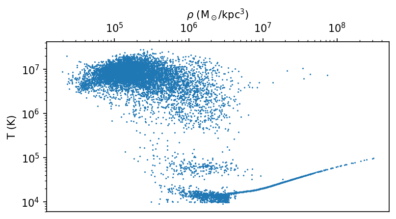
As we often use large datasets, we need to be careful with the amount of data we plot. Generally, we reduce the data by either selecting a subset or reducing it prior to plotting. For example, we can select a subset of particles by applying a cut on a given field.

Selecting a subset of particles

from scida import load
import matplotlib.pyplot as plt

ds = load("./snapdir_030")
dens = ds.data["PartType0"]["Density"][:10000].to("Msun/kpc^3").magnitude.compute()  # (1)!
temp = ds.data["PartType0"]["Temperature"][:10000].to("K").magnitude.compute()

fig, ax = plt.subplots(figsize=(6, 3))
ax.plot(dens, temp, "o", markersize=0.5)
ax.set_xscale("log")
ax.set_yscale("log")
ax.set_xlabel(r"$\rho$ (M$_\odot$/kpc$^3$))")
ax.set_ylabel(r"T (K)")
ax.xaxis.tick_top()
ax.xaxis.set_label_position('top')
plt.show()

1. Note the subselection of the first 10000 particles and conversion to a numpy array. Replace this operation with a meaninguful selection operation (e.g. a certain spatial region selection).

Simple scatter plot.

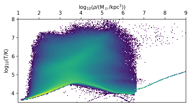
Instead of subselection, we sometimes want to visualize all of the data. We can do so by first applying reduction operations using dask. A common example would be a 2D histogram.

2D histograms

import dask.array as da
import numpy as np
from scida import load
import matplotlib.pyplot as plt
from matplotlib.colors import LogNorm

ds = load("./snapdir_030")
dens10 = da.log10(ds.data["PartType0"]["Density"].to("Msun/kpc^3").magnitude)
temp10 = da.log10(ds.data["PartType0"]["Temperature"].to("K").magnitude)

bins = [np.linspace(1, 9, 256 + 1), np.linspace(3.5, 8, 128 + 1)]
hist, xedges, yedges = da.histogram2d(dens10, temp10, bins=bins)
hist, xedges, yedges = hist.compute(), xedges.compute(), yedges.compute()
extent = [xedges[0], xedges[-1], yedges[0], yedges[-1]]

fig, ax = plt.subplots(figsize=(6,3))
ax.imshow(hist.T, origin="lower", extent=extent, aspect="auto", cmap="viridis",
          norm=LogNorm(), interpolation="none")
ax.set_xlabel(r"$\log_{10}$($\rho$/(M$_\odot$/kpc$^3$))")
ax.set_ylabel(r"$\log_{10}$(T/K)")
ax.xaxis.tick_top()
ax.xaxis.set_label_position('top')
plt.show()

Density-temperature phase-space diagram for TNG50-4

Interactive visualization

Info

This example requires the holoviews, datashader and bokeh packages installed. Make sure that these holoviews examples work before continuing.

We can do interactive visualization with holoviews. For example, we can create a scatter plot of the particle positions.

import holoviews as hv
import holoviews.operation.datashader as hd
import datashader as dshdr
from scida import load

ds = load("./snapdir_030")
ddf = ds.data["PartType0"].get_dataframe(["Coordinates0", "Coordinates1", "Masses"])  # (1)!

hv.extension("bokeh")
shaded = hd.datashade(hv.Points(ddf, ["Coordinates0", "Coordinates1"]), cmap="viridis", interpolation="linear",
                      aggregator=dshdr.sum("Masses"), x_sampling=5, y_sampling=5)
hd.dynspread(shaded, threshold=0.9, max_px=50).opts(bgcolor="black", xaxis=None, yaxis=None, width=500, height=500)

1. Visualization operations in holowview primarily run with dataframes, which we thus need to create using this wrapper for given fields.